Table of Contents
Turing Instabilities Part 2: Gierer-Meinhardt Model
The previous section derived the conditions that are needed for a Turing instability to exist. Now, let us step through an example in order to see how this works in practice.
We will consider the Gierer-Meinhardt model, which is a reaction diffusion system that describes an activator-inhibitor interaction. It is one of the equations that have been used to model morphogenesis and patterns in development, though experimental evidence is still lacking to support these models in full.
A slightly simplified version of the original Gierer-Meinhardt model [(gm_1972)] is,
\begin{gather} \label{eqn:gmor1} \frac{\partial u}{\partial t} = \frac{ u^2}{v} - bu + D_u \frac{\partial^2u}{\partial x^2}, \\ \label{eqn:gmor2} \frac{\partial v}{\partial t} = u^2 - v + D_v \frac{\partial^2v}{\partial x^2}. \end{gather}
where we will call u our “activator” and v our “inhibitor, $D_u$ and $D_v$ are diffusion constants, and $b$ is the rate at which the activator $u$ will naturally degrade.
Stability without Diffusion
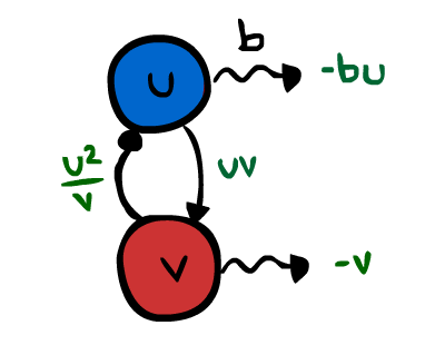
We can picture the diffusionless case of this system as the following picture, where the terms in the equation correspoding to the given connection are written in green:
Since the diffusionless model looks like, \begin{gather} \label{eqn:gmsta1} \frac{\partial u}{\partial t} = \frac{ u^2}{v} - bu, \\ \label{eqn:gmsta2} \frac{\partial h}{\partial t} = u^2 - v, \end{gather}
We see that the steady state is given by $u_0 = 1/b$ and $v_0 = u_0^2 = 1/b^2$. Linearizing about the steady state $[u_0, v_0] = [1/b, 1/b^2]$ (i.e. by Taylor expanding about the steady state and ignoring higher order terms), we obtain that the Jacobian is,
\begin{equation} \left.J\right|_{(1/b, 1/b^2)} = \left. \left(\begin{array}{cc} -b + \frac{2u}{v} & - \frac{u^2}{v^2} \\ 2u & -1 \end{array} \right) \right|_{(1/b, 1/b^2)} = \left(\begin{array}{cc} b & - b^2 \\ \frac{2}{b} & -1 \end{array} \right). \end{equation}
We then check that it is stable recalling from the previous section that this means $tr(J) <0$ and $det(J) >0$. Therefore we require that,
- $tr(J) = b-1 < 0$ so $b<1$
- $det(J) = b >0$ so $b>0$
This constrains the value of the parameter $b$ to $0<b<1$.
Instability with diffusion
When we add diffusion to the system we want it to be unstable. The way we look at this is by starting at the steady state and adding a small perturbation, and what we want is for these perturbations to grow over time.
Let $u(x,t) = u_0 + \tilde{u}$ and $v(x,t) = v_0 + \tilde{v}$, with $\tilde{u}$ and $\tilde{v}$ very small. Then, we look at the linearised system to study $\frac{\partial \tilde{u}}{\partial t}$ and $\frac{\partial \tilde{v}}{\partial t}$.
The linearised system looks like \begin{gather} \label{eqn:gmLin1} \frac{\partial \tilde{u}}{\partial t} = b\tilde{u} - b^2 \tilde{v}+ D_u \frac{\partial^2\tilde{u}}{\partial x^2}, \\ \label{eqn:gmLin2} \frac{\partial \tilde{v}}{\partial t} = \frac{2}{b} \tilde{u} - \tilde{v} + D_v \frac{\partial^2\tilde{v}}{\partial x^2}. \end{gather}
The system can be solved by separation of variables as we saw in the previous example, so we look for solutions of the form, \begin{equation} \label{eqn:SepSol} \binom{\tilde{u}}{\tilde{v}} =\binom{ A(t)e^{iqx} }{B(t)e^{iqx}}, \end{equation} where q are the Fourier modes.
The system becomes, \begin{equation} \label{JacobianPert} \frac{\partial}{\partial t} \binom{\delta\tilde{u}}{\delta \tilde{v}} = \left( \begin{array}{cc} b - q^2D_u & -b^2 \\ \frac{2}{b} & -1-q^2D_v \end{array} \right) \binom{\delta\tilde{u}}{\delta\tilde{v}} \end{equation}
We want to find the eigenvalues $\lambda_{1,2}$ of the $2\times2$ matrix, and we want them to be distinct, and at least one of $Re(\lambda_i) > 0$, $i\in\{1,2\}$. Notice that $tr(J) = b-1 - q^2(D_u+D_v)$ is always negative since $b<1$ by our condition above, and $D_u$, $D_v$ are both positive by definition, this condition is always true. In order for the system to become unstable, we need, \begin{equation} det(J) = H(q^2) = (b - D_uq^2)(-1-D_vq^2) +2b <0 \end{equation}


Notice that the determinant is a quadratic function with respect to $q^2$. In the gif above you can see a graph of $H$ for different values of b between $0$ and $0.35$. We will not get patterns for small values of b, but we will get patterns once the quadratic crosses the x-axis (i.e. has real nonnegative roots).
We will get two real roots for the quadratic when,
\begin{equation} -bD_v+D_u > 2\sqrt{(D_uD_v)b}. \end{equation}
Spatial Domain
If we apply periodic boundary conditions over a domain $x\in [0,L]$, the separable solution will then be of the form \begin{equation} \label{eqn:sumFour} \sum_k A_k e^{\lambda(q^2)t} cos(qx), \end{equation} and over the allowed values of k i.e. \begin{equation} q = \frac{n\pi}{L}, n \in \{1,2,...\}. \end{equation}
Since we want patterns to form, then the smallest allowed $L$ has to be such that \begin{equation} q^2 = \frac{\pi^2}{L^2} > \frac{A + \sqrt{A^2-B}}{2D_uD_v} = q^2_+, \end{equation} where $A = bD_v -D_u$, $B = 4bD_uD_v$, and $q^2_+$ is the bigger of the two solutions of $H(q^2)$. In other words, our critical length will be $L_c = \frac{\pi}{q_+}$.
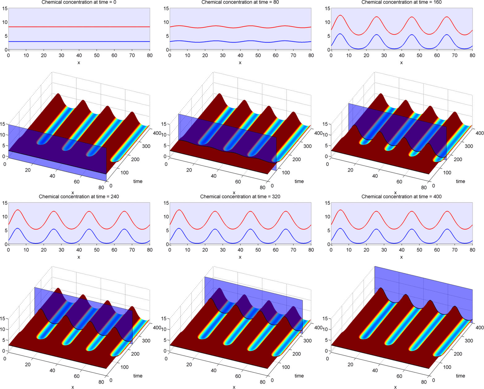
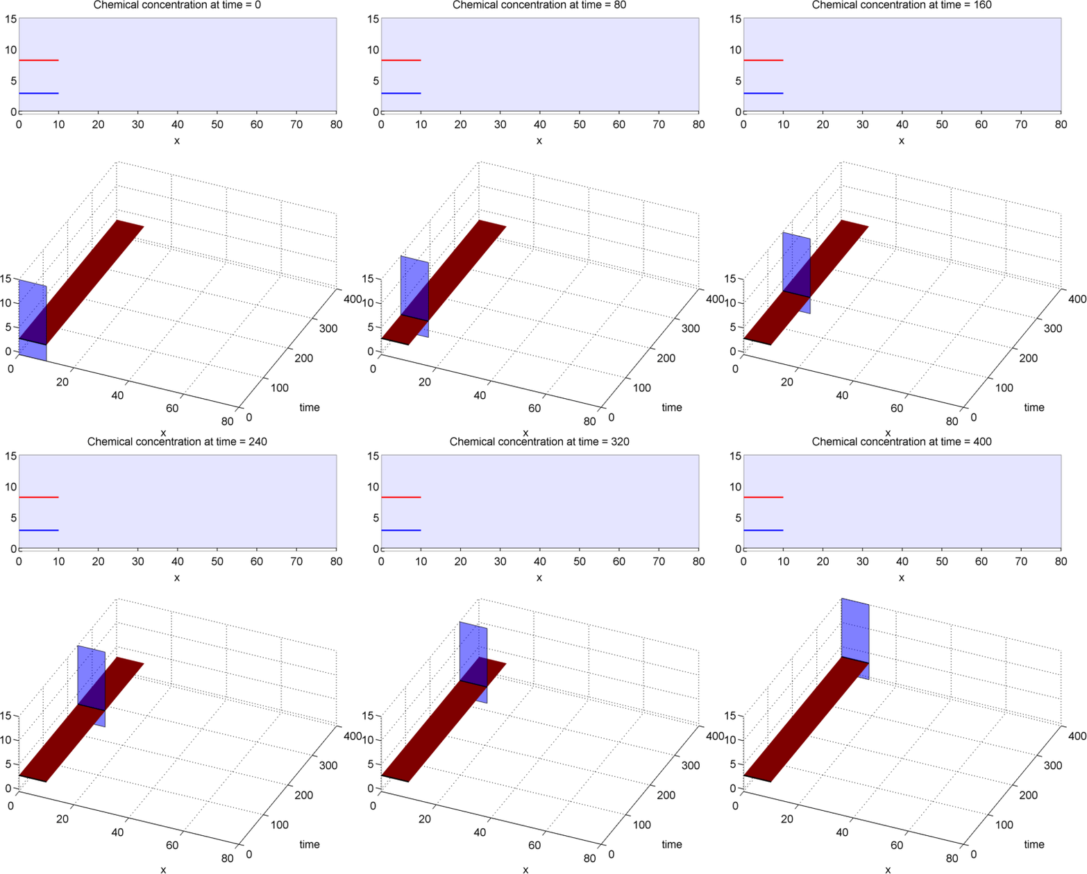
The two animations visualize the spatial dependence of patterns. For both animations, the initial conditions are small perturbations away from the steady state. The first animation takes a length $L<L_c$, that leads to stable patterns. However, when we use a domain that is smaller than the critical length $L<L_c$, no patterns will form. (Note that even though this is a useful visualization of our discussion above, in practice, it is difficult to numerically guarantee that “nothing” will happen)
You can now proceed to the next chapter: Turing Instabilities III
References
[(:gm_1972» author: Gierer A. and Meinhardt H. ref-author: Gierer and Meinhardt title: A theory of biological pattern formation journal: Kybernetic volume: 12 year: 1972 )]


